This package provides tools to propagate orbital states with different methods.
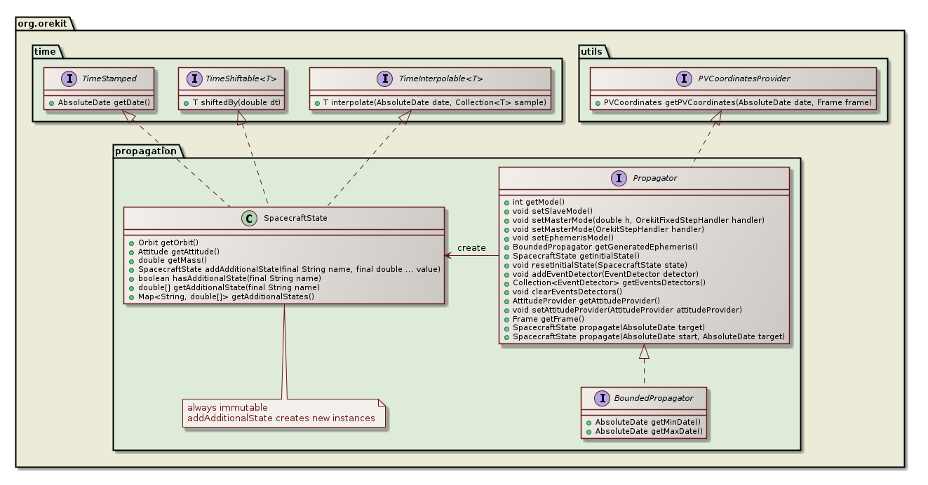
Propagation is the prediction of the evolution of a system from an initial state. In Orekit, this initial state is represented by a SpacecraftState, which is a simple container for all needed information : orbit, mass, kinematics, attitude, date, frame, and which can also hold any number user-defined additional data like battery status or operating mode for example.
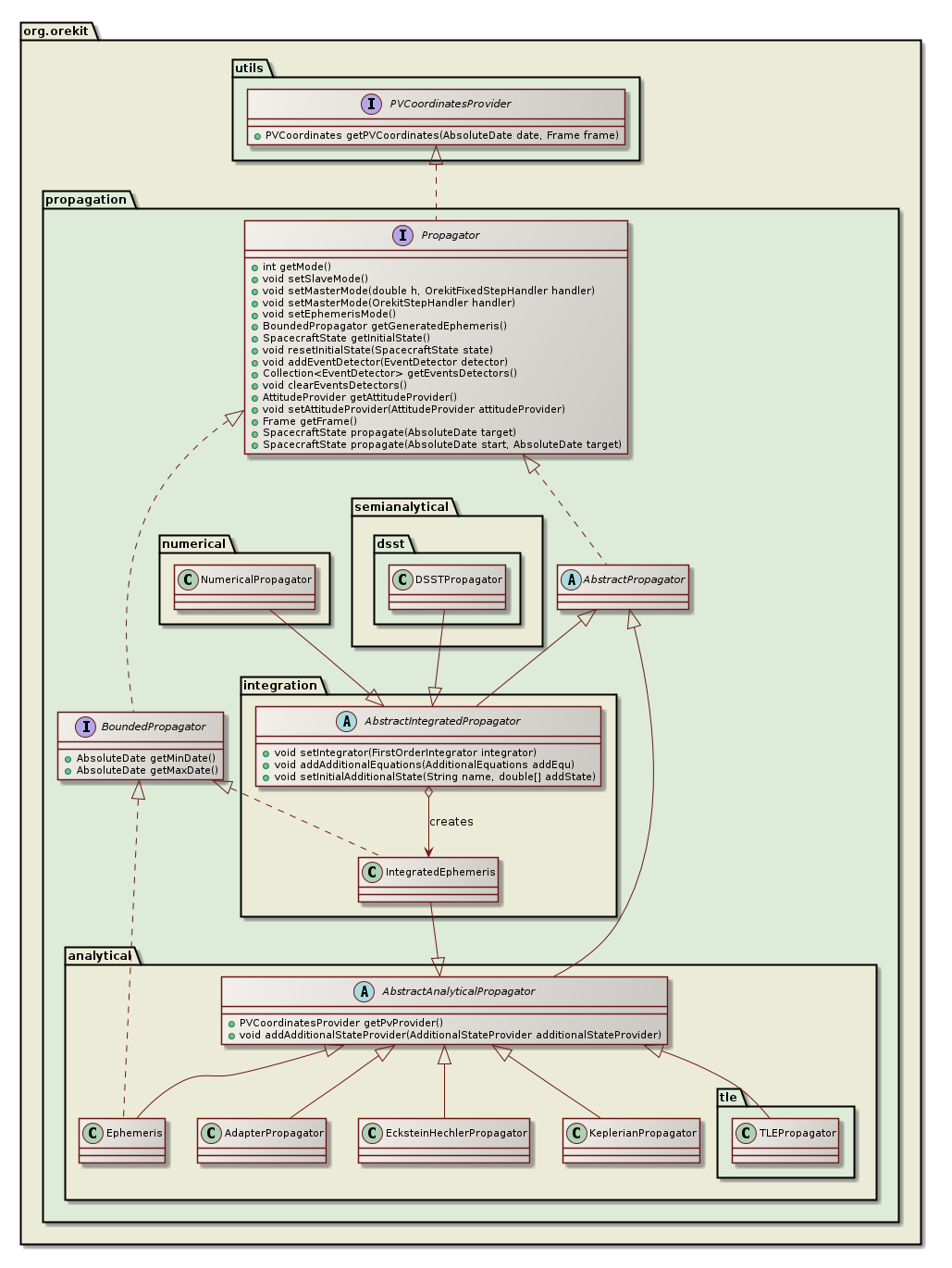
Propagation is based on a top level Propagation interface (which in facts extends the PVCoordinatesProvider interface) and several implementations.
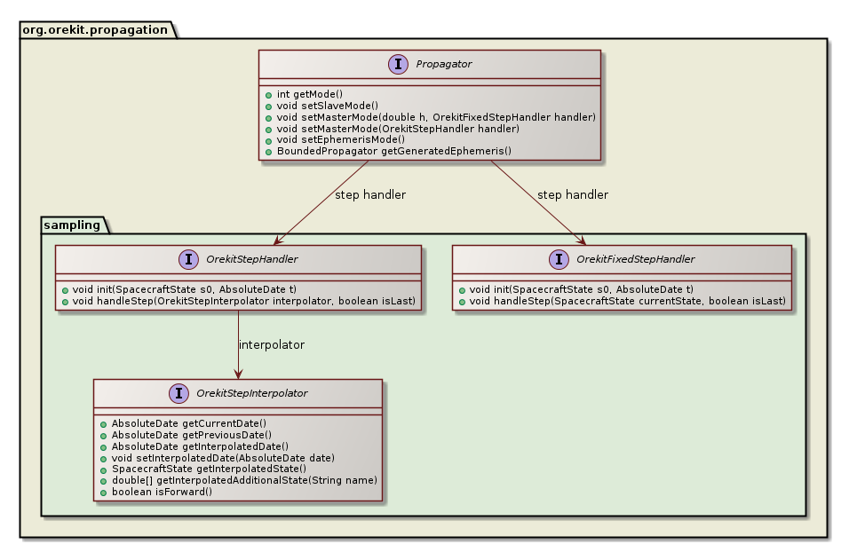
Depending on the needs of the calling application, all propagators can be used in different modes:
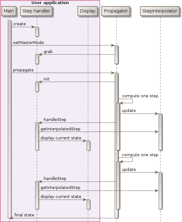
The recommended mode is master mode. It is very simple to use and allow user to get rid of concerns about synchronizing force models, file output, discrete events. All these parts are handled separately in different user code parts, and Orekit takes care of all management. The following class diagram shows the main interfaces used for master mode.
This mode also lets the propagator choose its own step size, but still let user choose a different step size for its output, which greatly increases performances. The following sequence diagram shows how a user-provided step handler is called when propagation is done in master mode.
The following sequence diagram shows how user can handle themselves time when propagation is done in slave mode, with a loop managed at user level.

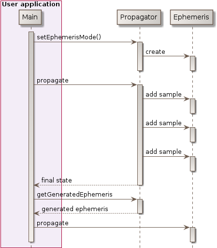
The following sequence diagram shows how user can use ephemeris generation mode to do a two phases propagation, one first phase to generate the epehemeris, and a second phase using the generated ephemeris.
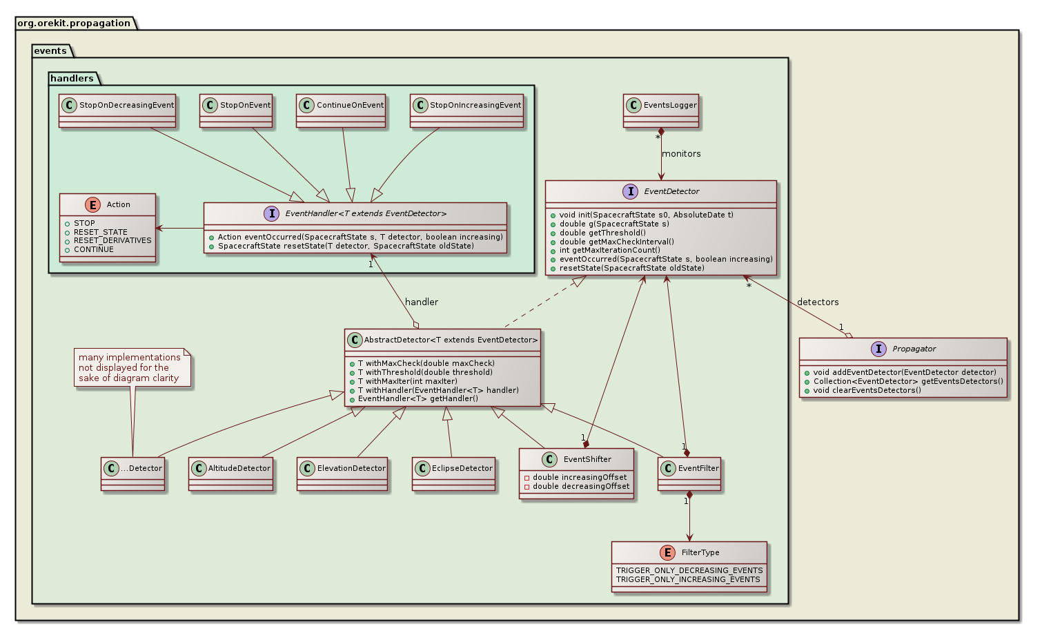
All propagators, including analytical ones, support discrete events handling during propagation. This feature is activated by registering events detectors as defined by the EventDetector interface to the propagator, each EventDetector being associated with an EventHandler that will be triggered automatically at event occurrence. The following class diagram shows the main interfaces used for event handling.
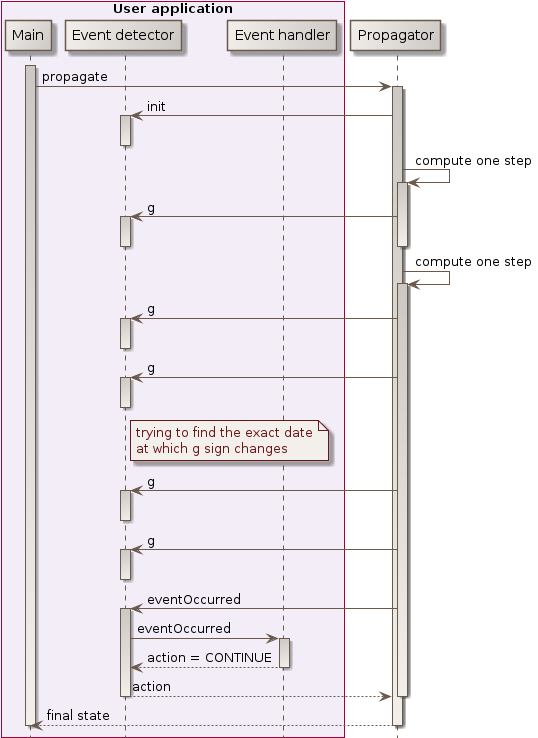
At each propagation step, the propagator checks the registered events detectors for the occurrence of some event, as shown in the following sequence diagram. If an event occurs, then the corresponding action is triggered, which can notify the propagator to resume propagation (possibly with an updated state) or to stop propagation.
Resuming propagation with changed state is used for example in the ImpulseManeuver class. When the maneuver is triggered, the orbit is changed according to the velocity increment associated with the maneuver and the mass is reduced according to the consumption. This allows the handling simple maneuvers transparently even inside basic propagators like Kepler or Eckstein-Heschler.
Stopping propagation is useful when some specific state is desired but its real occurrence time is not known in advance. A typical example would be to find the next ascending node or the next apogee. In this case, we can register a NodeDetector or an ApsideDetector object and launch a propagation with a target time far away in the future. When the event is triggered, it notifies the propagator to stop and the returned value is the state exactly at the event time.
Users can define their own events, typically by extending the AbstractDetector abstract class. There are also several predefined events detectors already available, amongst which :
An EventShifter is also provided in order to slightly shift the events occurrences times. A typical use case is for handling operational delays before or after some physical event really occurs.
An EventFilter is provided when user is only interested in one kind of events that occurs in pairs like raising in the raising/setting pair for elevation detector, or eclipse entry in the entry/exit pair for eclipse detector. The filter does not simply ignore events after they have been detected, it filters them before they are located and hence save some computation time by not doing an accurate search for events that will ultimately be ignored.
Event occurring can be automatically logged using the EventsLogger class.
All propagators can be used to propagate user additional states on top of regular orbit attitude and mass state. These additional states will be available throughout propagation, i.e. they can be used in the step handlers, in the event detectors and events handlers and they will also be available in the final propagated state. There are three main cases:
The first two cases correspond to additional states managed by the propagator, the last case not being considered as managed. The list of states managed by the propagator is available using the getManagedAdditionalStates and isAdditionalStateManaged.
The KeplerianPropagator is based on Keplerian-only motion. It depends only on µ.
This analytical model is suited for near-circular orbits and inclination neither equatorial nor critical. It considers J2 to J6 potential zonal coefficients, and uses mean parameters to compute the new position.
Note that before version 7.0, there was a large inconsistency in the generated orbits. It was fixed as of version 7.0 of Orekit, with a visible side effect. The problem is that if the circular parameters produced by the Eckstein-Hechler model are used to build an orbit considered to be osculating, the velocity deduced from this orbit was inconsistent with the position evolution! The reason is that the model includes non-Keplerian effects but it does not include a corresponding circular/Cartesian conversion. As a consequence, all subsequent computation involving velocity were wrong. This includes attitude modes like yaw compensation and Doppler effect. As this effect was considered serious enough and as accurate velocities were considered important, the propagator now generates Cartesian orbits which are built in a special way to ensure consistency throughout propagation. A side effect is that if circular parameters are rebuilt by user from these propagated Cartesian orbit, the circular parameters will generally not match the initial orbit (differences in semi-major axis can exceed 120 m). The position however will match to sub-micrometer level, and this position will be identical to the positions that were generated by previous versions (in other words, the internals of the models have not been changed, only the output parameters have been changed). The correctness of the initialization has been assessed and is good, as it allows the subsequent orbit to remain close to a numerical reference orbit.
If users need a more definitive initialization of an Eckstein-Hechler propagator, they should consider using a propagator converter to initialize their Eckstein-Hechler propagator using a complete sample instead of just a single initial orbit.
This model is used to add to an underlying propagator some effects it does not take into account. A typical example is to add small station-keeping maneuvers to a pre-computed ephemeris or reference orbit which does not take these maneuvers into account. The additive maneuvers can take both the direct effect (Keplerian part) and the induced effect due for example to J2 which changes ascending node rate when a maneuver changed inclination or semi-major axis of a Sun-Synchronous satellite.
Numerical propagation is one of the most important parts of the Orekit project. Based on Apache Commons Math ordinary differential equations integrators, the NumericalPropagator class realizes the interface between space mechanics and mathematical resolutions. Despite its utilization seems daunting on first sight, it is in fact quite straigthforward to use.
The mathematical problem to integrate is a dimension-seven time-derivative equations system. The six first elements of the state vector are the orbital parameters, which may be any orbit type (KeplerianOrbit, CircularOrbit, EquinoctialOrbit or CartesianOrbit) in meters and radians, and the last element is the mass in kilograms. It is possible to have more elements in the state vector if AdditionalEquations have been added (typically PartialDerivativesEquations which is an implementation of AdditionalEquations devoted to integration of Jacobian matrices). The time derivatives are computed automatically by the Orekit using the Gauss equations for the first parameters corresponding to the selected orbit type and the flow rate for mass evolution during maneuvers. The user only needs to register the various force models needed for the simulation. Various force models are already available in the library and specialized ones can be added by users easily for specific needs.
The integrators (first order integrators) provided by Apache Commons Math need the state vector at t0, the state vector first time derivative at t0, and then calculates the next step state vector, and asks for the next first time derivative, etc. until it reaches the final asked date. These underlying numerical integrators can also be configured. Typical tuning parameters for adaptive stepsize integrators are the min, max and perhaps start step size as well as the absolute and/or relative errors thresholds. The following code snippet shows a typical setting for Low Earth Orbit propagation:
// steps limits
final double minStep  = 0.001;
final double maxStep  = 1000;
final double initStep = 60;

// error control parameters (absolute and relative)
final double positionError = 10.0;
final double[][] tolerances = NumericalPropagator.tolerances(positionError, orbit, orbit.getType());

// set up mathematical integrator
AdaptiveStepsizeIntegrator integrator =
    new DormandPrince853Integrator(minStep, maxStep, tolerances[0], tolerances[1]);
integrator.setInitialStepSize(initStep);

// set up space dynamics propagator
propagator = new NumericalPropagator(integrator);
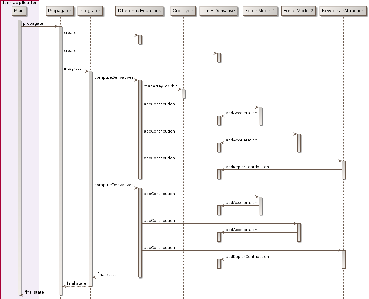
The following sequence diagram show the internal calls triggered during a numerical propagation. The important thing to note is that the force model are decoupled from the integration process, they only need to compute an acceleration.
Sometimes, simple equations of motion are not enough. Some additional parameters can be useful alongside with the trajectory, like dual parameters in optimal control or Jacobians (also called state-transition matrices). This second case especially useful for computing sensitivity of a trajectory with respect to initial state changes or with respect to force models parameters changes.
Orekit provides a common way to handle both cases: additional equations. Users can register sets of additional equations alongside with additional initial states. These equations will be propagated by the numerical integrator. They will not be used for step control, though, so integrating with or without these equations should not change the trajectory and no tolerance setting is needed for them.
One specific implementation of additional equations is the partial derivatives equations which propagate Jacobian matrices, both with respect to initial state and with respect to force model parameters.
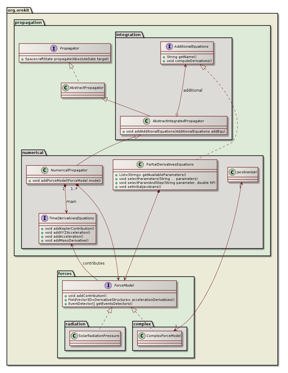
The above class diagram shows the design of the partial derivatives equations. As can be seen, the PartialDerivativesEquations class implements the AdditionalEquations interface and as such can be registered by user in a numerical propagator. the propagator will propagate both the main set of equations corresponding to the equations of motion and the additional set corresponding to the Jacobians of the main set. This additional set is therefore tightly linked to the main set and in particular depends on the selected force models. The various force models add their direct contribution directly to the main set, just as in simple propagation. They also add a contribution to the Jacobians thanks to the AccelerationJacobiansProvider interface, each force model being associated with an acceleration Jacobians provider. Some force models like solar radiation pressure implement this interface by themselves. Some more complex force model do not implement the interface and will be automatically wrapped inside a Jacobianizer class which will use finite differences to compute the local Jacobians.
Semianalytical propagation is an intermediate between analytical and numerical propagation. It retains the best of both worlds, speed from analytical models and accuracy from numerical models. Semianalytical propagation is implemented using Draper Semianalytical Satellite Theory (DSST).
Since version 7.0, both mean elements equations of motion modelsand short periodic terms have been implemented and validated.