
The org.orekit.estimation package provides classes to manage orbit determination.
Orbit determination support in Orekit is similar to other space flight dynamics topics support: the library provides the framework with top level interfaces and classical implementations (say distance and angular measurements among others). Some hooks are also provided for expert users who need to supplement the framework with mission-specific features and implementations (say specific delay models for example). The provided objects are sufficient for basic orbit determination and can easily be extended to address more operational needs.
There are two main sub-packages: org.orekit.estimation.measurements and org.orekit.estimation.leastsquares.

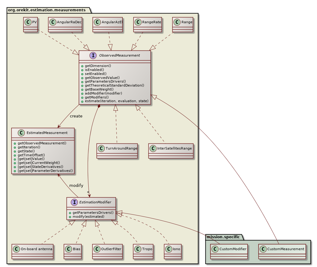
The measurements package defines everything that is related to the measurements themselves, both the theoretical values and the modifications that can be applied to them. All measurements must implement the ObservedMeasurement interface, which is the public API that the engine will use to deal with all measurements. The most important methods of this interface allow to:
The estimated measurements can be modified by registering one or several EstimationModifier objects. These objects will manage notions like ionospheric or tropospheric delays, biases, ground antennas position offsets, Antenna Phase Center… One specific modifier OutlierFilter can be used to reject outliers at run time if the current residuals exceed the theoretical standard deviation by some user-defined factor.
A typical operational case from a ground stations network would create distance and angular measurements, create one bias modifier for the on-board delay for distance measurements, a few modifiers for each ground station (position offset, delay), modifiers for tropospheric and ionospheric delays and add them to corresponding measurements (i.e. all distance measurements would share the same on-board delay object, but distance measurements performed by two difference ground stations would refer to different sets of ground station positions offsets for example).
The classical measurements and modifiers are already provided by Orekit in the same package, but for more advanced needs, users are expected to implement their own implementations. This ensures the extensibility of this design.

The leastsquares package provides an implementation of a batch least squares estimator engine to perform an orbit determination. Users will typically create one instance of this object, register all observation data as measurements with their included modifiers, and run the least squares filter. At the end of the process, a fully configured propagator is returned, including the estimated orbit as the initial state and the estimated propagator parameters. The estimated measurement and propagator parameters can also be retrieved by themselves.
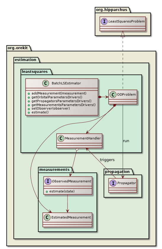
The BatchLSEstimator class creates an internal implementation of Hipparchus LeastSquaresProblem interface to represent the orbit determination problem and passes it to one of the LeastSquaresOptimizer implementations to solve it. Several choices are possible, among which LevenbergMarquardtOptimizer and GaussNewtonOptimizer. The former is considered more robust and can start from initial guesses farther than the second one. If GaussNewtonOptimizer is neverthelesss selected, it should be configured to use QR decomposition rather than LU decomposition for increased stability in case of poor observability. During the resolution, the selected Hipparchus algorithm will call the evaluate method of the local LeastSquaresProblem model at each algorithm test point. This will trigger one orbit propagation with some test values for the orbit state and the parameters (for example biases from the measurements modifiers parameters or drag coefficients from the force models parameters). During the propagation, the Orekit step handler mechanism is used to collect the state and its Jacobians at measurements dates. A MeasurementHandler class performs the binding between the generic step handling mechanism and the orbit determination framework. At each measurement date, it gets the state and Jacobians from the propagator side, calls the measurement methods to get the residuals and the partial derivatives on the measurements side, and fetches the least squares estimator with the combined values, to be provided back to the Hipparchus least squares solver, thus closing the loop.
Users can decide what they want to estimate. The 6 orbital parameters are typically always estimated and are selected by default, but it is possible to fix some or all of these parameters. Users can also estimate some propagator parameters (like drag coefficient or radiation pressure coefficients) and measurements parameters (like biases, stations position offsets or Earth Orientation parameters). One use case for estimating only a subset of the orbital parameters is when observations are very scarce (say the first few measurements on a newly detected debris or asteroid). One use case for not estimating any orbital parameters at all is when calibrating measurements biases from a reference orbit considered to be perfect. Selecting which parameters should be estimates and which parameters should remain fixed is done thanks to the ParameterDriver class. During setup, the user can retrieve three different ParametersDriversList from the BatchLSEstimator:
Then, looping on the elements of these lists, the user can change the default settings depending on his/her needs and for example fix a few orbital parameters while estimating a few propagation and measurements parameters.
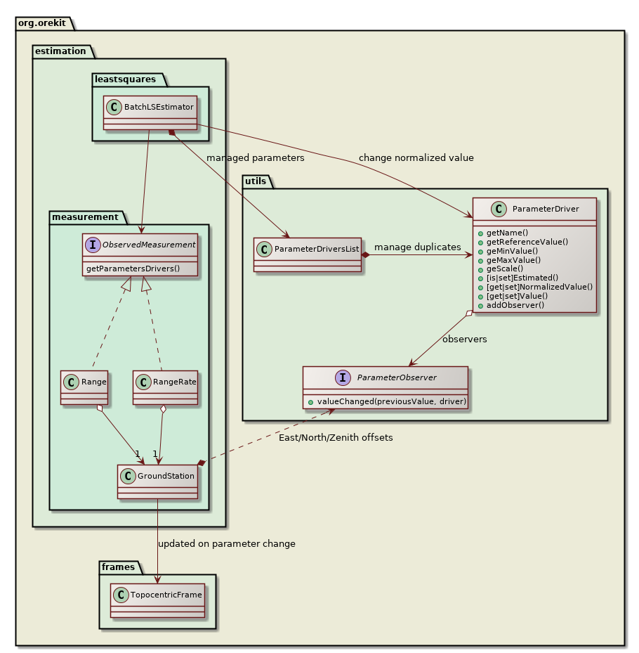
Once everything has been set up, the estimate method of BatchLSEstimator is called. The least squares solver will then modify the values of the parameters that have been flagged as selected (and hence should be estimated). The estimator does not know the meaning of any of the parameters, they appear all the same for it. Under the hood, each parameters was in fact created by an object which knows what the parameter mean, like for example an object involved in the drag computation. This object uses the observer design pattern to monitor each change attempted by the optimization algorithm, and it will adapt its computation according to the last change performed. This design improves the decoupling between the upper layer managing the batch least square estimation and the lower layer to which force models or biases belong. It therefore allows user to add their own parameters if they create specific force models, specific measurements or specific measurements modifiers. All they need to do is provide some ParameterDriver instances and implement the ParameterObserver interface to monitor when the estimator will change these new parameters.

The class diagram above depicts the parameter update mechanism for the case of ground station position offset. The Range and RangeRate measurements classes refer to a GroundStation instance (one instance shared by all measurements using this station) that provides to the upper layer 3 parameters representing the East, North and Zenith offset for station position. If some station position offset is flagged to be estimated, the BatchLSEstimator will change its value at each new evaluation, without knowing what this change really involves underneath. As the parameters values are changed, the ground station will be notified of the change thanks to the ParameterObserver it did register to the parameters, and it moves its associated TopocentricFrame according to the updated offsets. The Range and RangeRate measurements theoretical values will therefore be computed naturally using the updated station position. Orbital parameters, propagation parameters and measurements parameters are all handled the same way.
Parameters normalization is used to present a more balanced vector to the least squares algorithm. Without normalization, the vector component corresponding to the semi-major axis would have an order of magnitude of a few millions whereas the vector component corresponding to the eccentricity would be 10 orders of magnitude smaller (assuming user decided to estimate an orbit in Keplerian parameters set). If central attraction coefficient were estimated, the discrepancy between the largest and smallest component could even reach 20 orders of magnitudes. Least squares optimizers do not handle such vectors properly. In order to cope with this problem, the mathematical least squares algorithm only sees normalized values for parameters, while the physical models see real values for the same parameters. The normalized value is always computed as:
normalized = (physical - reference) / scale
The reference value and the scale are fixed. The scale is related to the expected excursion around reference that can be expected in a typical problem. It is not really important to have it precisely computed as the goal is only to avoid huge orders of magnitudes. Any scale that allows the normalized value to be somewhere between 1/1000 and 1000 is good enough. For this reason, the scale is hard-coded for each parameter. In order to increase numerical stability, the hard-coded values are powers of 2 so sequences of multiplications and divisions when converting between normalized and physical values do not introduce computation errors. As an example, the scale factor for drag coefficient has been set to 2⁻³ whereas the scale factor for central attraction coefficient has been set to 2⁺³².
Some parameters values are forbidden and should not be used by the least squares estimator. Unfortunately, as of mid 2017 the Hipparchus library does not support simple bounds constraints for these algorithms. There is however a workaround with parameters validator. Orekit uses this workaround and set up a validator for the full set of parameters. This validator checks the test values provided by the least squares solver are within the parameters bounds, and if not it simply force them at boundary, effectively clipping the values. Just like scaling factors, the minimum and maximum bounds are currently hard-coded in the library. The limits have been set to quite loose value, as they are only meant to prevent computation failures (like negative eccentricities or semi-major axes). If anyway the least squares algorithm tries such extreme values, there is probably a problem with either the measurements or the propagator configuration.